This data was collected from the LaGuardia Airport station in New York City for October 2018. It contains: - the daily minimum temperature (TMIN) - the daily maximum temperature (TMAX) - the daily average temperature (TAVG)
Note: The NCEI is part of the National Oceanic and Atmospheric Administration (NOAA) and, as you can see from the URL for the API, this resource was created when the NCEI was called the NCDC. Should the URL for this resource change in the future, you can search for “NCEI weather API” to find the updated one.
In addition, we will be using S&P 500 stock market data (obtained using the stock_analysis package and data for bitcoin for 2017 through 2018. For the first edition, the bitcoin data was collected from CoinMarketCap using the stock_analysis package; however, changes in the website led to the necessity of changing the data source to Yahoo! Finance. The bitcoin data that was collected before the CoinMarketCap website change should be equivalent to the historical data that can be viewed on this page.
Setup
We need to import pandas and read in the temperature data to get started:
import pandas as pddf = pd.read_csv('../data/nyc_temperatures.csv')df.head()
We want to rename the value column to indicate it contains the temperature in Celsius and the attributes column to say flags since each value in the comma-delimited string is a different flag about the data collection. For this task, we use the rename() method and pass in a dictionary mapping the column names to their new names. We pass inplace=True to change our original dataframe instead of getting a new one back:
This also works with Series/DataFrame objects that have an index of type DatetimeIndex. Let’s read in the CSV again for this example and set the date column to be the index and stored as a datetime:
We can use tz_convert() to convert to another timezone from there. If we convert the Eastern datetimes to UTC, they will now be at 5 AM, since pandas will use the offsets to convert:
eastern.tz_convert('UTC').head()
datatype
station
attributes
value
date
2018-10-01 05:00:00+00:00
TAVG
GHCND:USW00014732
H,,S,
21.2
2018-10-01 05:00:00+00:00
TMAX
GHCND:USW00014732
,,W,2400
25.6
2018-10-01 05:00:00+00:00
TMIN
GHCND:USW00014732
,,W,2400
18.3
2018-10-02 05:00:00+00:00
TAVG
GHCND:USW00014732
H,,S,
22.7
2018-10-02 05:00:00+00:00
TMAX
GHCND:USW00014732
,,W,2400
26.1
We can change the period of the index as well. We could change the period to be monthly to make it easier to aggregate later.
The reason we have to add the parameter within tz_localize() to None for this, is because we’ll get a warning from pandas that our output class PeriodArray doesn’t have time zone information and we’ll lose it.
We can use the assign() method for working with multiple columns at once (or creating new ones). Since our date column has already been converted, we need to read in the data again:
date        datetime64[ns]
datatype            object
station             object
flags               object
temp_C             float64
temp_F             float64
dtype: object
The date column now has datetimes and the temp_F column was added:
new_df.head()
date
datatype
station
flags
temp_C
temp_F
0
2018-10-01
TAVG
GHCND:USW00014732
H,,S,
21.2
70.16
1
2018-10-01
TMAX
GHCND:USW00014732
,,W,2400
25.6
78.08
2
2018-10-01
TMIN
GHCND:USW00014732
,,W,2400
18.3
64.94
3
2018-10-02
TAVG
GHCND:USW00014732
H,,S,
22.7
72.86
4
2018-10-02
TMAX
GHCND:USW00014732
,,W,2400
26.1
78.98
We can also use astype() to perform conversions. Let’s create columns of the integer portion of the temperatures in Celsius and Fahrenheit. We will use lambda functions (first introduced in Chapter 2, Working with Pandas DataFrames), so that we can use the values being created in the temp_F column to calculate the temp_F_whole column. It is very common (and useful) to use lambda functions with assign():
Say we want to find the days that reached the hottest temperatures in the weather data; we can sort our values by the temp_C column with the largest on top to find this:
However, this isn’t perfect because we have some ties, and they aren’t sorted consistently. In the first tie between the 7th and the 10th, the earlier date comes first, but the opposite is true with the tie between the 4th and the 2nd. We can use other columns to break ties and specify how to sort each with ascending. Let’s break ties with the date column and show earlier dates before later ones:
Notice that the index was jumbled in the past 2 results. Here, our index only stores the row number in the original data, but we may not need to keep track of that information. In this case, we can pass in ignore_index=True to get a new index after sorting:
The sample() method will give us rows (or columns with axis=1) at random. We can provide a seed (random_state) to make this reproducible. The index after we do this is jumbled:
df.sample(5, random_state=0).index
Index([2, 30, 55, 16, 13], dtype='int64')
We can use sort_index() to order it again:
df.sample(5, random_state=0).sort_index().index
Index([2, 13, 16, 30, 55], dtype='int64')
The sort_index() method can also sort columns alphabetically:
df.sort_index(axis=1).head()
datatype
date
flags
station
temp_C
temp_C_whole
temp_F
temp_F_whole
0
TAVG
2018-10-01
H,,S,
GHCND:USW00014732
21.2
21
70.16
70
1
TMAX
2018-10-01
,,W,2400
GHCND:USW00014732
25.6
25
78.08
78
2
TMIN
2018-10-01
,,W,2400
GHCND:USW00014732
18.3
18
64.94
64
3
TAVG
2018-10-02
H,,S,
GHCND:USW00014732
22.7
22
72.86
72
4
TMAX
2018-10-02
,,W,2400
GHCND:USW00014732
26.1
26
78.98
78
This can make selection with loc easier for many columns:
Now that we have an index of type DatetimeIndex, we can do datetime slicing and indexing. As long as we provide a date format that pandas understands, we can grab the data. To select all of 2018, we simply use df.loc['2018'], for the fourth quarter of 2018 we can use df.loc['2018-Q4'], grabbing October is as simple as using df.loc['2018-10']; these can also be combined to build ranges. Let’s grab October 11, 2018 through October 12, 2018 (inclusive of both endpoints)—note that using loc[] is optional for ranges:
df['2018-10-11':'2018-10-12']
datatype
station
flags
temp_C
temp_C_whole
temp_F
temp_F_whole
date
2018-10-11
TAVG
GHCND:USW00014732
H,,S,
23.4
23
74.12
74
2018-10-11
TMAX
GHCND:USW00014732
,,W,2400
26.7
26
80.06
80
2018-10-11
TMIN
GHCND:USW00014732
,,W,2400
21.7
21
71.06
71
2018-10-12
TAVG
GHCND:USW00014732
H,,S,
18.3
18
64.94
64
2018-10-12
TMAX
GHCND:USW00014732
,,W,2400
22.2
22
71.96
71
2018-10-12
TMIN
GHCND:USW00014732
,,W,2400
12.2
12
53.96
53
We can also use reset_index() to get a fresh index and move our current index into a column for safe keeping. This is especially useful if we had data, such as the date, in the index that we don’t want to lose:
df['2018-10-11':'2018-10-12'].reset_index()
date
datatype
station
flags
temp_C
temp_C_whole
temp_F
temp_F_whole
0
2018-10-11
TAVG
GHCND:USW00014732
H,,S,
23.4
23
74.12
74
1
2018-10-11
TMAX
GHCND:USW00014732
,,W,2400
26.7
26
80.06
80
2
2018-10-11
TMIN
GHCND:USW00014732
,,W,2400
21.7
21
71.06
71
3
2018-10-12
TAVG
GHCND:USW00014732
H,,S,
18.3
18
64.94
64
4
2018-10-12
TMAX
GHCND:USW00014732
,,W,2400
22.2
22
71.96
71
5
2018-10-12
TMIN
GHCND:USW00014732
,,W,2400
12.2
12
53.96
53
Reindexing allows us to conform our axis to contain a given set of labels. Let’s turn to the S&P 500 stock data in the sp500.csv file to see an example of this. Notice we only have data for trading days (weekdays, excluding holidays):
If we want to look at the value of a portfolio (group of assets) that trade on different days, we need to handle the mismatch in the index. Bitcoin, for example, trades daily. If we sum up all the data we have for each day (aggregations will be covered in chapter 4, so don’t fixate on this part), we get the following:
bitcoin = pd.read_csv('../data/bitcoin.csv', index_col='date', parse_dates=True).drop(columns=['market_cap'])# every day's closing price = S&P 500 close + Bitcoin close (same for other metrics)portfolio = pd.concat([sp, bitcoin], sort=False).groupby(level='date').sum()portfolio.head(10).assign( day_of_week=lambda x: x.index.day_name())
high
low
open
close
volume
day_of_week
date
2017-01-01
1003.080000
958.700000
963.660000
998.330000
147775008
Sunday
2017-01-02
1031.390000
996.700000
998.620000
1021.750000
222184992
Monday
2017-01-03
3307.959883
3266.729883
3273.170068
3301.670078
3955698000
Tuesday
2017-01-04
3432.240068
3306.000098
3306.000098
3425.480000
4109835984
Wednesday
2017-01-05
3462.600000
3170.869951
3424.909932
3282.380000
4272019008
Thursday
2017-01-06
3328.910098
3148.000059
3285.379893
3179.179980
3691766000
Friday
2017-01-07
908.590000
823.560000
903.490000
908.590000
279550016
Saturday
2017-01-08
942.720000
887.250000
908.170000
911.200000
158715008
Sunday
2017-01-09
3189.179990
3148.709902
3186.830088
3171.729902
3359486992
Monday
2017-01-10
3194.140020
3166.330020
3172.159971
3176.579902
3754598000
Tuesday
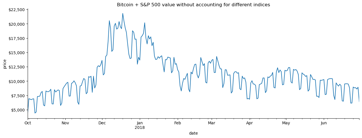
It may not be immediately obvious what is wrong with the previous data, but with a visualization we can easily see the cyclical pattern of drops on the days the stock market is closed. (Don’t worry about the plotting code too much, we will cover it in depth in chapters 5 and 6).
We will need to import matplotlib now:
import matplotlib.pyplot as plt # we use this module for plottingfrom matplotlib.ticker import StrMethodFormatter # for formatting the axis
Now we can see why we need to reindex:
# plot the closing price from Q4 2017 through Q2 2018ax = portfolio['2017-Q4':'2018-Q2'].plot( y='close', figsize=(15, 5), legend=False, title='Bitcoin + S&P 500 value without accounting for different indices')# formattingax.set_ylabel('price')ax.yaxis.set_major_formatter(StrMethodFormatter('${x:,.0f}'))for spine in ['top', 'right']: ax.spines[spine].set_visible(False)# show the plotplt.show()
We need to align the index of the S&P 500 to match bitcoin in order to fix this. We will use the reindex() method, but by default we get NaN for the values that we don’t have data for:
So now we have rows for every day of the year, but all the weekends and holidays have NaN values. To address this, we can specify how to handle missing values with the method argument. In this case, we want to forward-fill, which will put the weekend and holiday values as the value they had for the Friday (or end of trading week) before:
To isolate the changes happening with the forward-filling, we can use the compare() method. It shows us the values that differ across identically-labeled dataframes (same names and same columns). Here, we can see that only weekends and holidays (Monday, January 16, 2017 was MLK day) have values forward-filled. Notice that consecutive days have the same values.
This isn’t perfect though. We probably want 0 for the volume traded and to put the closing price for the open, high, low, and close on the days the market is closed:
The reason why we’re using np.where(boolean condition, value if True, value if False) within lambda functions in the example below, is that vectorized operations allow us to be faster and more efficient than utilizing for loops to perform calculations on arrays all at once.
import numpy as npsp_reindexed = sp.reindex(bitcoin.index).assign( volume=lambda x: x.volume.fillna(0), # put 0 when market is closed close=lambda x: x.close.fillna(method='ffill'), # carry this forward# take the closing price if these aren't availableopen=lambda x: np.where(x.open.isnull(), x.close, x.open), high=lambda x: np.where(x.high.isnull(), x.close, x.high), low=lambda x: np.where(x.low.isnull(), x.close, x.low))sp_reindexed.head(10).assign( day_of_week=lambda x: x.index.day_name())
high
low
open
close
volume
day_of_week
date
2017-01-01
NaN
NaN
NaN
NaN
0.000000e+00
Sunday
2017-01-02
NaN
NaN
NaN
NaN
0.000000e+00
Monday
2017-01-03
2263.879883
2245.129883
2251.570068
2257.830078
3.770530e+09
Tuesday
2017-01-04
2272.820068
2261.600098
2261.600098
2270.750000
3.764890e+09
Wednesday
2017-01-05
2271.500000
2260.449951
2268.179932
2269.000000
3.761820e+09
Thursday
2017-01-06
2282.100098
2264.060059
2271.139893
2276.979980
3.339890e+09
Friday
2017-01-07
2276.979980
2276.979980
2276.979980
2276.979980
0.000000e+00
Saturday
2017-01-08
2276.979980
2276.979980
2276.979980
2276.979980
0.000000e+00
Sunday
2017-01-09
2275.489990
2268.899902
2273.590088
2268.899902
3.217610e+09
Monday
2017-01-10
2279.270020
2265.270020
2269.719971
2268.899902
3.638790e+09
Tuesday
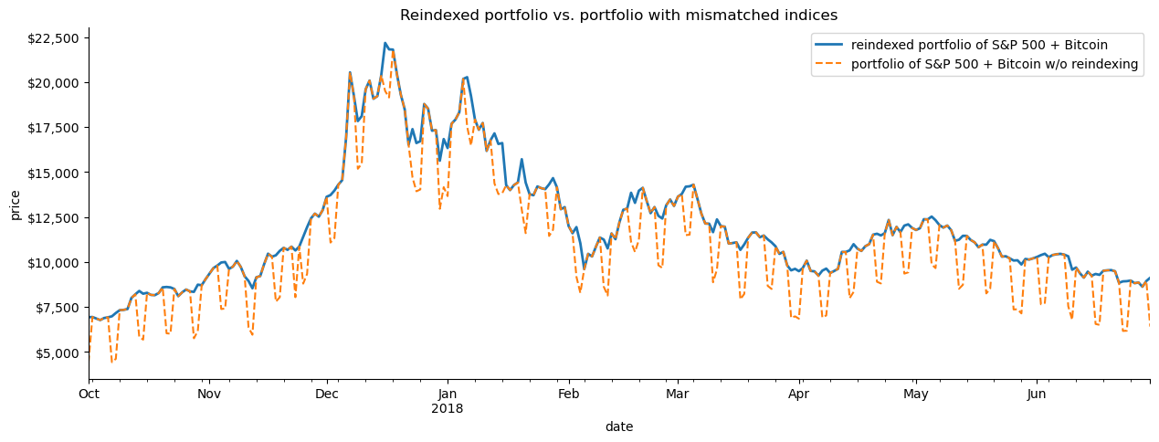
If we create a visualization comparing the reindexed data to the first attempt, we see how reindexing helped maintain the asset value when the market was closed:
# every day's closing price = S&P 500 close adjusted for market closure + Bitcoin close (same for other metrics)fixed_portfolio = sp_reindexed + bitcoin# plot the reindexed portfolio's closing price from Q4 2017 through Q2 2018ax = fixed_portfolio['2017-Q4':'2018-Q2'].plot( y='close', label='reindexed portfolio of S&P 500 + Bitcoin', figsize=(15, 5), linewidth=2, title='Reindexed portfolio vs. portfolio with mismatched indices')# add line for original portfolio for comparisonportfolio['2017-Q4':'2018-Q2'].plot( y='close', ax=ax, linestyle='--', label='portfolio of S&P 500 + Bitcoin w/o reindexing')# formattingax.set_ylabel('price')ax.yaxis.set_major_formatter(StrMethodFormatter('${x:,.0f}'))for spine in ['top', 'right']: ax.spines[spine].set_visible(False)# show the plotplt.show()